Learn tsmap
Yield tells you how many dies passed. The measurements behind it tell you how close to their limits the dies were. This lesson shows how test values spread, how groups of wafers compare, and where to find the numbers behind every chart.
This tab is about how values spread: process capability, a box plot per wafer, a histogram and the trend across wafers. It answers "are my tests healthy, or close to failing?"
Which wafers behave differently from the rest? At the top of Distributions, Tests by wafer picks the tests whose wafers differ most and draws them as a grid. Each row is a test and each column is a wafer.
The colour of a cell shows how far that wafer's mean is from the mean of all the wafers: blue is below, orange is above, and a pale cell is close to average.
Each cell needs a common scale, so that millivolts and megahertz can sit side by side.
How much room does each test have before it fails? Each test is rescaled against its own limits: the low limit becomes 0 and the high limit becomes 1. That puts tests in different units on one scale, so you can compare their margins directly.
Each test is a box showing where its values sit between the limits.
A test without both limits still appears, drawn muted and dashed on its own range, with no Ppk. Its place says how its values spread, not how near a limit they are, because there is no limit to be near.
Under the heading Test by test there is one Test menu. Changing it changes the box plot, the histogram, the trend and the scatter together, so every card is about the same test and you can read them as one story.
A lot can have hundreds of tests. Click the ☆ at the end of a row in any test menu, or press P on the focused row, to pin that test. Pinned tests are listed first, under Pinned, in every test menu in Insights, and tsmap remembers them for the next lot.
Clicking a test in the capability chart does the same. A card shows a Test menu of its own only while you have expanded it.
1 Axis includes limits widens the axis to the limits. 2 Clip outliers narrows it to the bulk of the data. 3 Log scale, on the box plot only, uses a log axis once every value is positive.
Clipping does not remove data. The chart states how many values fall outside the axis, and every statistic still includes them.
When a test has both kinds, a Limits choice appears on the box plot, histogram, trend and scatter: Test + spec (the default), Test limits, Spec limits or None. A limit off the edge of the axis is marked with an arrow.
The histogram has a Wafer menu: all wafers pooled, or one wafer. Type to filter the list.
Is the process drifting from wafer to wafer? This chart shows each wafer's mean in slot order, with a band of ±1 standard deviation. There is no sort, because a drift only shows in sequence.
Control chart shows the same wafers against control limits, with the points that break a rule marked.
The two views answer different questions. The trend shows how the dies within each wafer spread. The control chart shows whether a wafer's mean stands out from the others, and it needs at least three wafers.
With Group by on, each group's bars are a share of its own dies, so groups of different sizes compare by shape rather than by size. Counts shows the number of dies instead.
Cumulative draws the same values as a curve instead of bars. Each die sits at the share of dies at or below its value, on a scale where a normal distribution falls on a straight line. A group whose curve is further right has higher values, and a steeper curve is a tighter spread.
With Group by on, the box plot also offers Split, then wafer: each split's wafers sit inside it, coloured by split, so you see the spread between splits and within each.
The box plot can show one box for each wafer (By wafer) or one for each ring, from the centre of the wafer out to the edge (By radius). By radius is the one to use when you suspect a value changes with distance from the centre: the boxes then step up or down from Ring 1 to Ring 4.
Comparing groups raises a fair question: why not use every die? Because the dies are not independent.
When you compare groups, the table gives you three things to read.
With Group by on, Tests by wafer becomes Tests by split: one column for each group instead of each wafer, in z-scores again. A group that is dark across several rows differs on several tests at once, which suggests one cause.
Grouped by Temperature, the card compares the six wafers tested at 85 °C with the nineteen at 25 °C. At 85 °C leakage (ioff_nA) is high, while the thresholds and both idsat_n_uA and fmax_MHz are lower.
ioff_nA
idsat_n_uA
fmax_MHz
Tester, program revision and burn-in time each pick out a different set of wafers. Group by each in turn to see which tests it moves.
Once you know two groups differ, the next question is where. The difference map shows where on the wafer two groups differ, not whether the difference is significant. Use the comparison table for that.
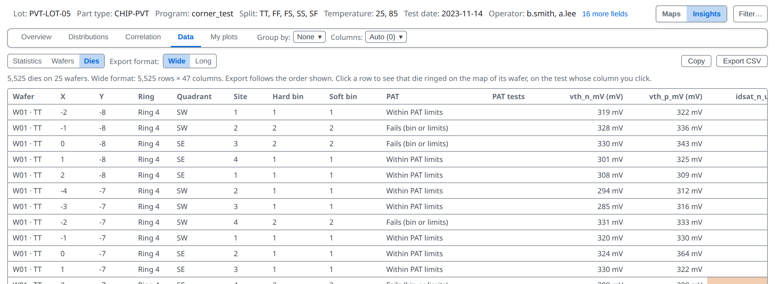
Every chart is drawn from numbers, and you can have them. Data, the tab after Correlation, holds every number behind the charts as tables. The foot of the Overview links to it too.
The Data tab holds the same numbers as tables, in three sub-tabs: Statistics, Wafers and Dies. Statistics has two tables, each with its own CSV button: 1 Test values CSV and 2 Functional CSV.
The Wafers table has one row per wafer: its lot fields, die counts, yield and the mean of each test.
The Dies table has one row per die: position, ring, quadrant, site, bins, every test and the PAT verdict. Copy puts it on the clipboard and Export CSV saves a file; Wide has a column per test, Long a row per die and test.
You can now say how a test behaves and whether groups differ. Next: which tests move together.
More in the wafer map guide
07 · Correlation →
Which tests move together.