Use cases¶

Four workflows tsmap is built for, written as procedures you can follow. Each states what it needs, what you should see, and — just as important — how to avoid over-reading the result.

New to tsmap? Start with the tutorial, which walks the first of these end to end on a bundled sample lot.

Yield triage across a lot¶

Use this when a lot has come off the prober and you need to know, quickly, whether its losses are random or structured.

You need: a multi-wafer STDF/ATDF file, or several single-wafer files opened together.

1. Open the lot. Import the tests you care about — bin and yield data is preserved regardless of the test selection, so you can select none and still do the whole of this workflow.
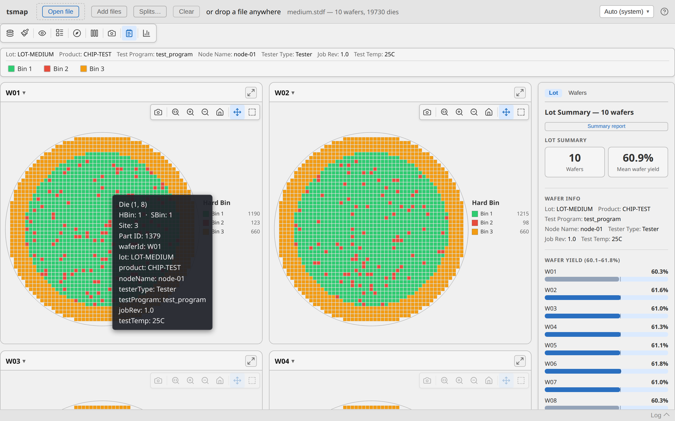
2. In the Summary panel (headed with the lot ID when every wafer shares one), read mean per-wafer yield and the Findings list.
3. Scroll to Wafer Yield and switch the Slot | Yield toggle to Yield. The list re-sorts worst-first.
4. Expand the worst wafer (⤢ on its card).
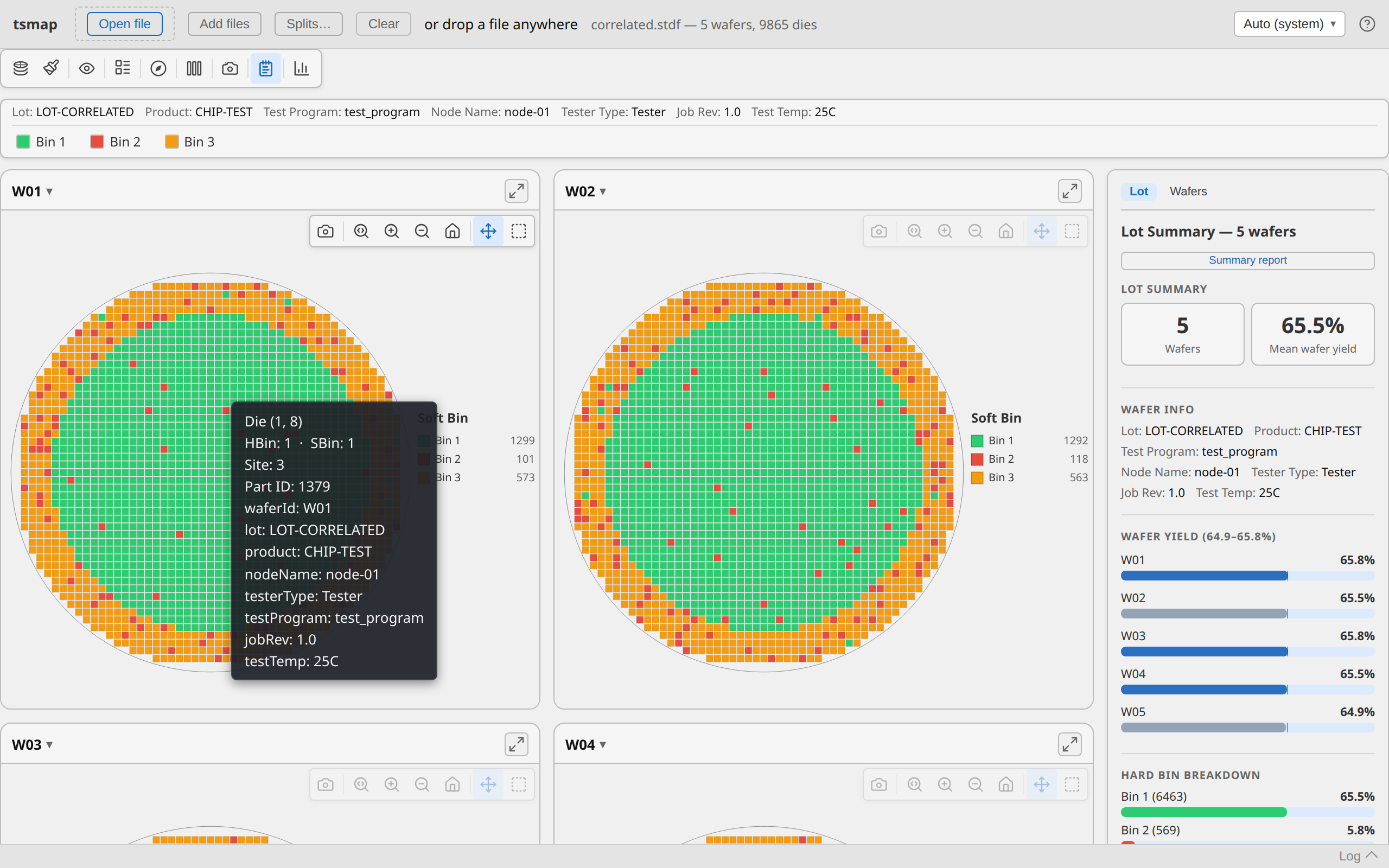
5. Set Plot mode → Soft Bin to resolve how the dies failed rather than just whether.

What you should see: a per-wafer yield ranking, and any spatial findings tsmap detected on its own — edge-local patterns, clustering, ring effects. Findings are always on; nothing needs configuring for them to appear.

Reading it correctly:

• Mean per-wafer yield is not lot yield. It is the arithmetic mean of per-wafer percentages, so a 50-die wafer counts as much as a 5,000-die one.
• A finding is a statistical statement, not a diagnosis. "Edge-local, medium confidence" means the edge dies fail more than the rest — not that the cause is the process. Probe-card contact, handling and chuck effects all produce edge signatures too.
• One bad wafer in thirteen may simply be one bad wafer. Look for whether the pattern repeats across wafers — findings report that as "seen on N/13 wafers".

Next: if the losses look structured, either group by split to see whether they track an experimental variable (below), or move to a parametric view to find which test is failing.

See Opening files and The wafer map view.

Root-causing a parametric fail via correlation¶

Use this when a specific parametric test is failing and you want to know whether it is failing on its own or moving with something else.

You need: a file with parametric (PTR) test values, and those tests imported — correlation needs the measured values, not just bins.

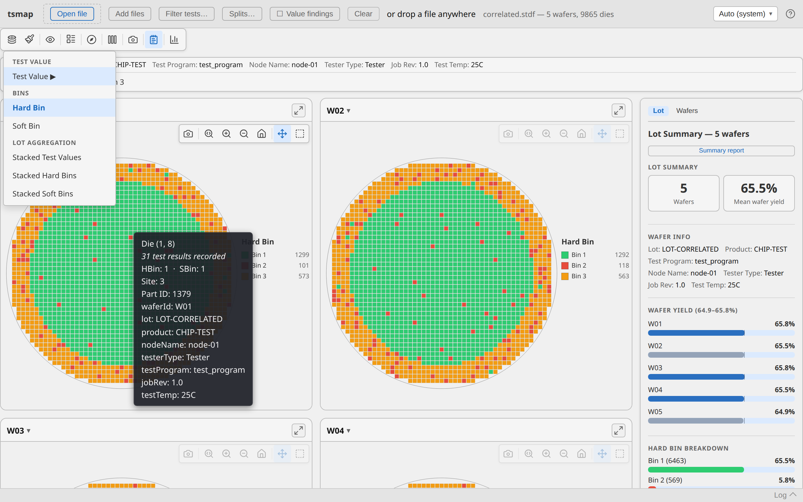
1. Set Plot mode → Test Value ▶ and pick the suspect test from the submenu. Tests are listed by name and unit, e.g. leakage_nA (nA). The map becomes a heat map of that measurement.
2. Open Insights and select the Correlation sub-tab.
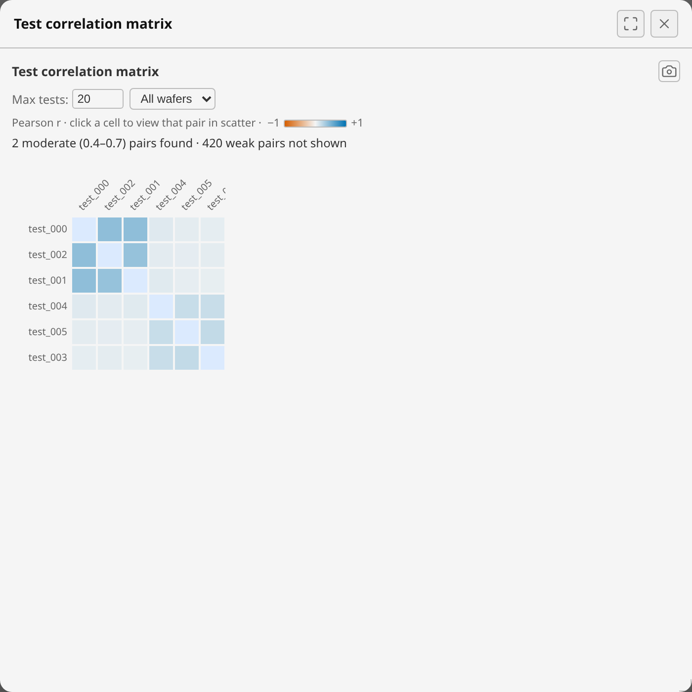
3. Read the Test correlation matrix. It reports Pearson r for every test pair, and states its own thresholds beneath the heading — for example "45 strong (|r| ≥ 0.7), 10 moderate (0.4–0.7) pairs found · 264 weak pairs not shown".
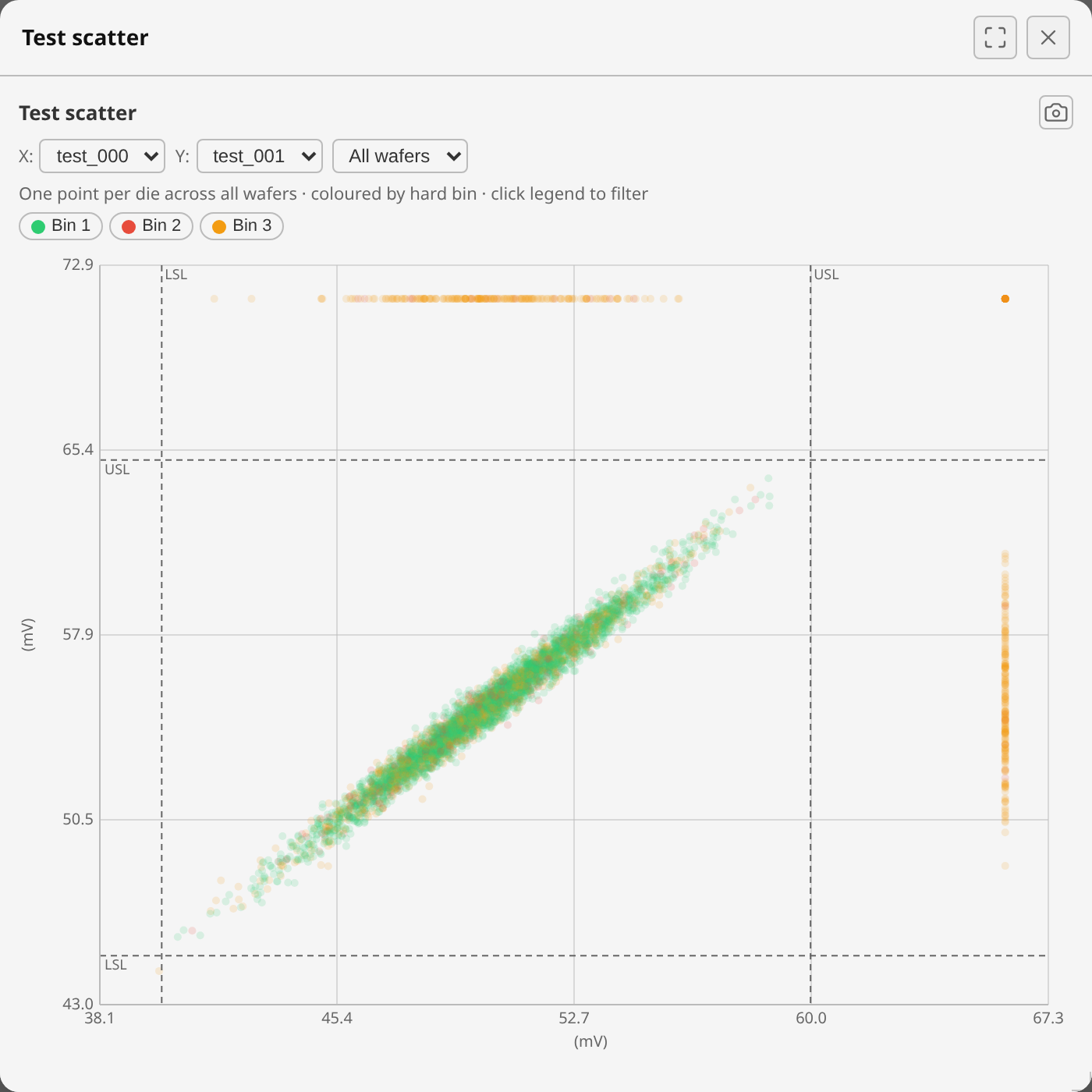
4. Click a matrix cell to load that pair into the Test scatter panel below it.
5. In the scatter, confirm the relationship is real: one point per die, coloured by hard bin, with r and n restated for the pair. Click a bin in the legend to filter to it.

What you should see: a matrix with your suspect test's row picked out, and a scatter that either shows a genuine trend or reveals that a high r came from something else.

Reading it correctly:

• Correlation is not causation, and here it is often not even a direct relationship. Two tests can track a third thing — temperature, die position, tester site — and correlate strongly without either influencing the other.
• Always look at the scatter, never the r alone. A single tight cluster plus a few outliers, or two separated groups, can both produce a high r that means nothing like what it appears to.
• Pooling wafers can manufacture correlation. r is computed across every die in scope by default; if two wafers sit at different offsets, that between-wafer separation alone creates a trend. Use the All wafers ▾ scope picker on either panel to re-check a single wafer. If the correlation vanishes, it was a between-wafer effect, not a per-die one.
• The matrix hides weak pairs and caps how many tests it shows (Max tests:) — an absent cell is not evidence of no relationship.

Next: if the correlation holds within a single wafer, check whether it also tracks a split (below). If it does not, the two tests are probably measuring the same physical mechanism.

See The wafer map view and Grouping data in the Insights tab.

Comparing process corners with splits¶

Use this when wafers in a lot were deliberately run differently and you need to compare the groups rather than the wafers.

You need: a lot whose wafers belong to known groups, and a record of which wafer is which.

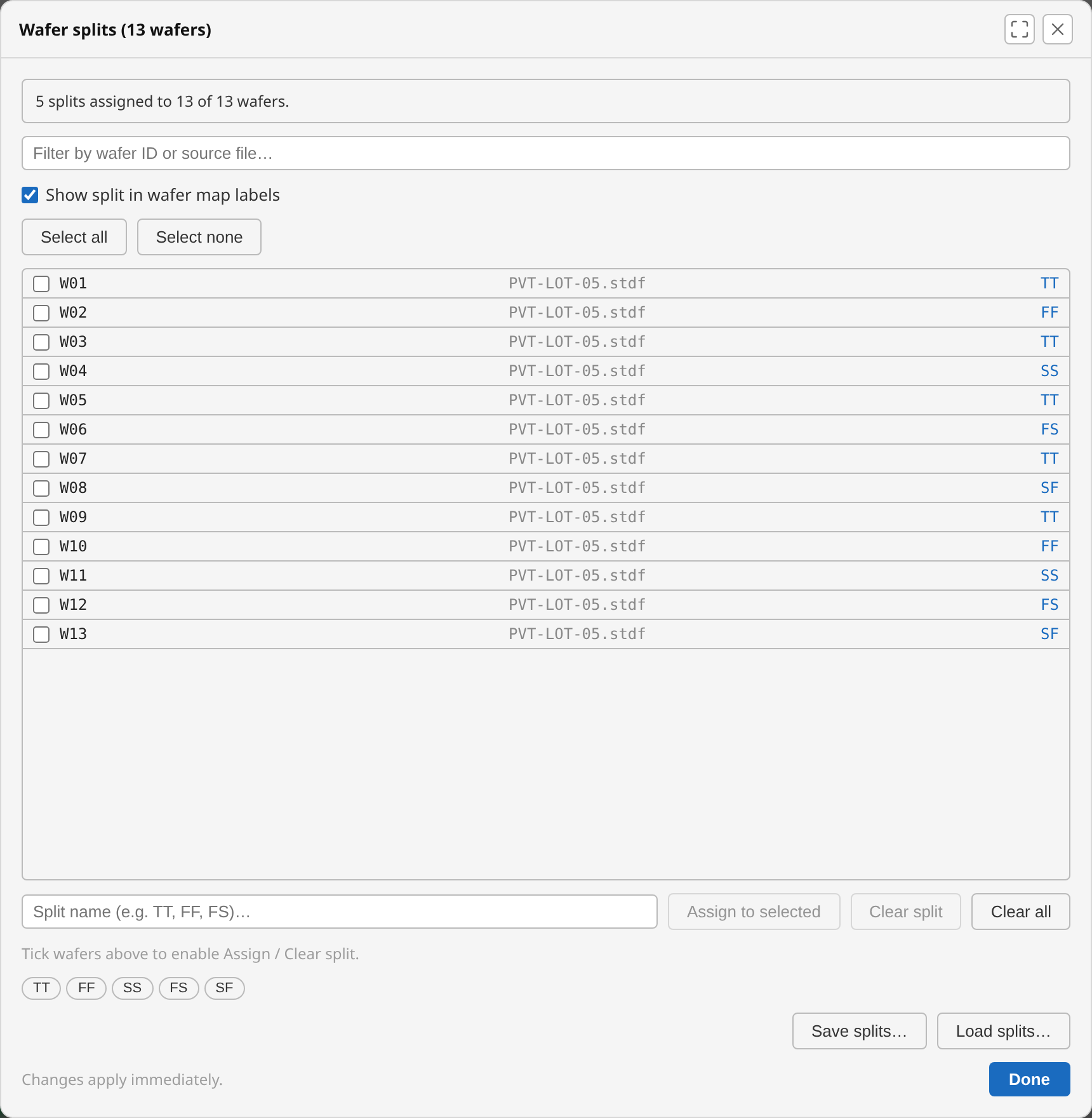
1. Open Setup ▾ → Splits….
2. Assign a label to each wafer (TT/FF/SS/FS/SF, or whatever your experiment uses), or load a splits CSV to assign them in bulk. Assignments are remembered per lot + wafer, so they survive a reload.
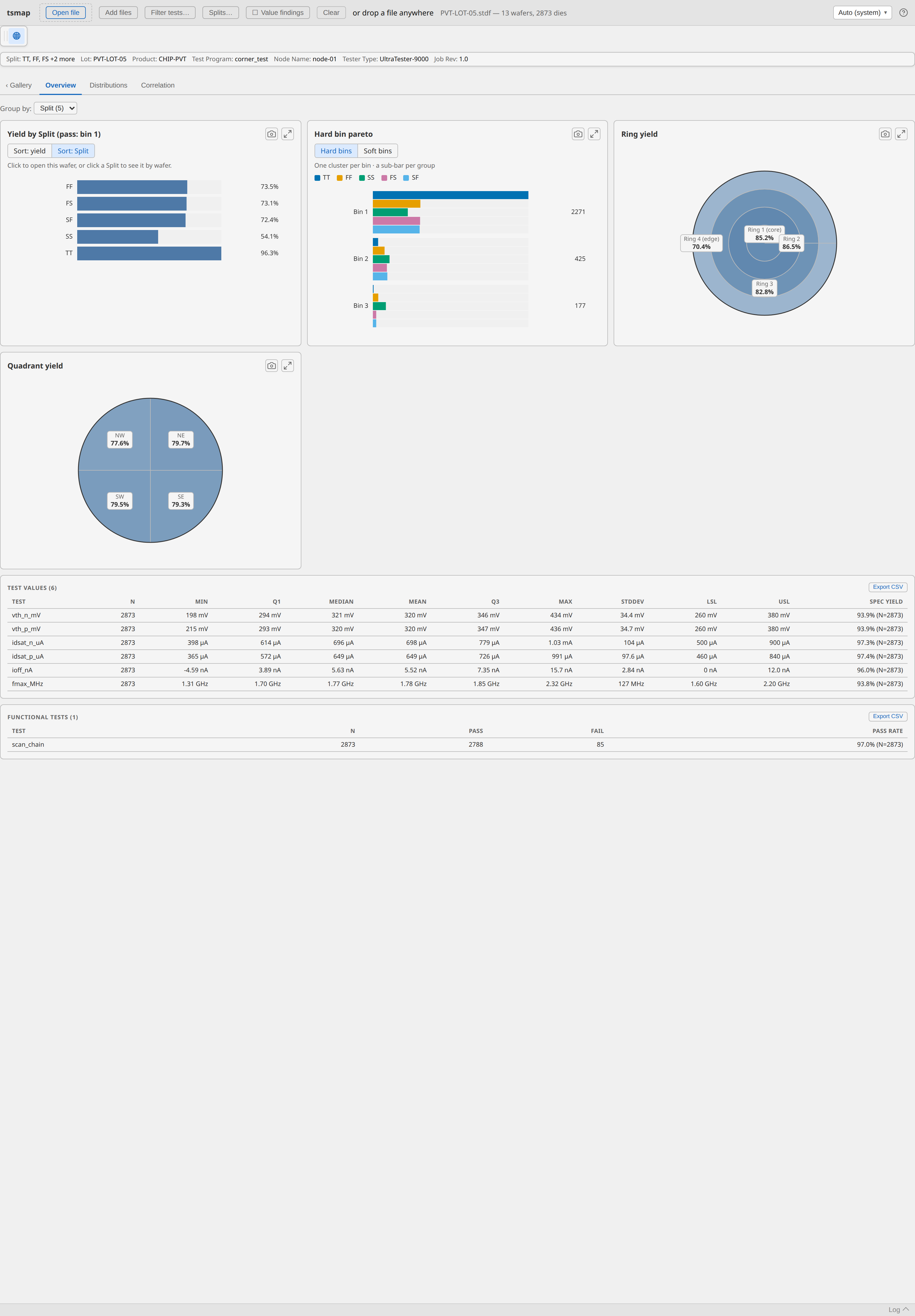
3. Close the dialog. Every gallery card is now suffixed with its split, e.g. W01 · TT.
4. Open Insights → Overview and set Group by: Split.
5. Read Yield by Split and the bin pareto side by side.
6. Click a bar in Yield by Split to drill into that corner's own wafers; ← Back returns.

What you should see: every Overview panel reported per corner instead of per wafer, so a corner effect that was spread across the slot order becomes a single ranked comparison.

Reading it correctly:

• Splits are your assertion, not the file's. Nothing validates them. One mislabelled wafer silently moves its dies into the wrong group and shifts both groups' numbers.
• Check the group sizes before believing the ranking. A corner represented by one wafer is one wafer, however it is plotted.
• A yield difference between corners says the groups differ — not which step caused it, and not that the corner is the only thing that varied between them.
• Look at which bins each corner loses dies to, not only how many. Two corners at the same yield failing into different bins are two different problems.

Next: drill into the worst corner's wafers and return to yield triage on those, or check whether a parametric test separates cleanly by corner in Distributions.

See Wafer splits.

Scripted and offline batch workflows¶

Use this when tsmap needs to open something chosen by another system, or when the data cannot leave the machine.

You need: the desktop app for the CLI flags; the browser build supports the URL form.

1. Open files directly: tsmap lot1.stdf lot2.stdf.
2. Supply a pre-built test selection with --tests. This pre-fills the test selector — checkboxes, renames and any limit/type overrides — but the overlay still appears and still needs a confirm click, exactly as it does for any other load. It saves re-picking the tests, not the click.
3. Seed wafer splits with --splits, so an experiment's grouping is applied on open.
4. To launch from another application, use a tsmap://open?url=…&format=… link (desktop) or ?dataUrl=…&dataFormat=… (browser). Both parameters are required together.

What you should see: the lot opens with its files, test selection and splits already applied — no file picker, and nothing to re-enter. The test selector still appears for you to confirm.

Reading it correctly:

• Parsing is entirely local on both platforms. Nothing is uploaded, so this is safe for confidential lot data and works with no network at all.
• The browser build fetches its dataUrl in the browser, so it is subject to the target server's CORS policy; the desktop app is not. This is the usual reason a link that works on the desktop fails in a tab.
• Do not put a long-lived API key in a launch URL — URLs persist in history, logs and referrer data. Use a short-lived URL, a same-origin gateway, or the desktop's --url-headers.

Next: Integrating data selection covers the full set of integration architectures and which ones avoid CORS entirely.

See Command line and Opening data from a URL.